Example walkthrough

This sections gives a walkthrough for analysing time-of-flight data for multiple frequency scans done as a sequence of increasing pressure conditions.

1. In the menu click File ‣ New project

   Select any suitable location for the project file and save the project file with a file extension .bz

2. In the menu click File ‣ Import ultrasound data ‣ Discrete f

   Navigate to and select the US folder containing subfolders with ultrasound frequency scans.

   Note

   The subfolders should contain oscilloscope waveform files from a frequency scan, sortable alha-numericaly from lowest to highest frequency. E.g. Exp4_25_C_2000_psi_29000_khz, sam1_001.csv. Avoid placing any extraneous subfolders or files in the US folder.

   Note

   The name of the subfolders will be displayed as the names of P-T conditions in the exported results table

   

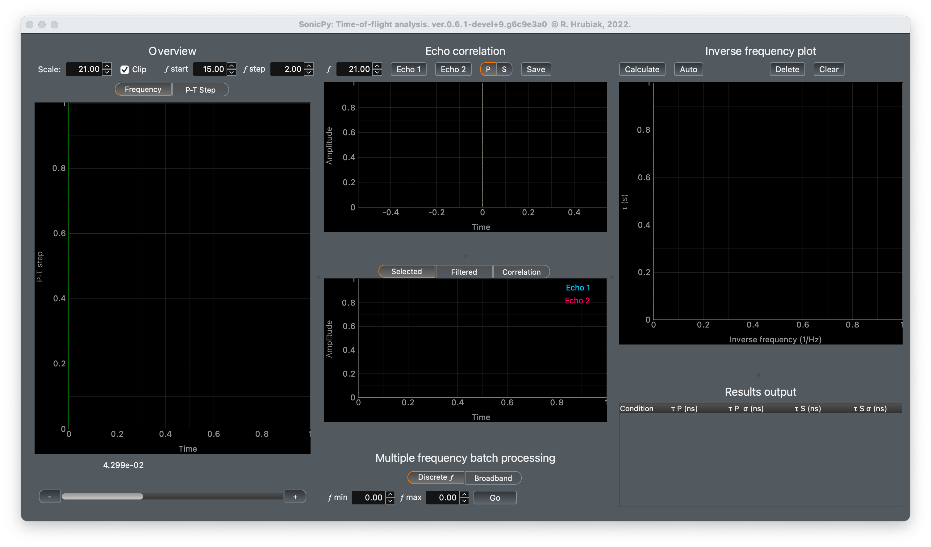
3. Enter \(f\) start and \(f\) step at the top of the Overview section, based on your experimental settings. The program uses the \(f\) start and \(f\) step values to calculate the frequency of each corresponding waveform.

   Note

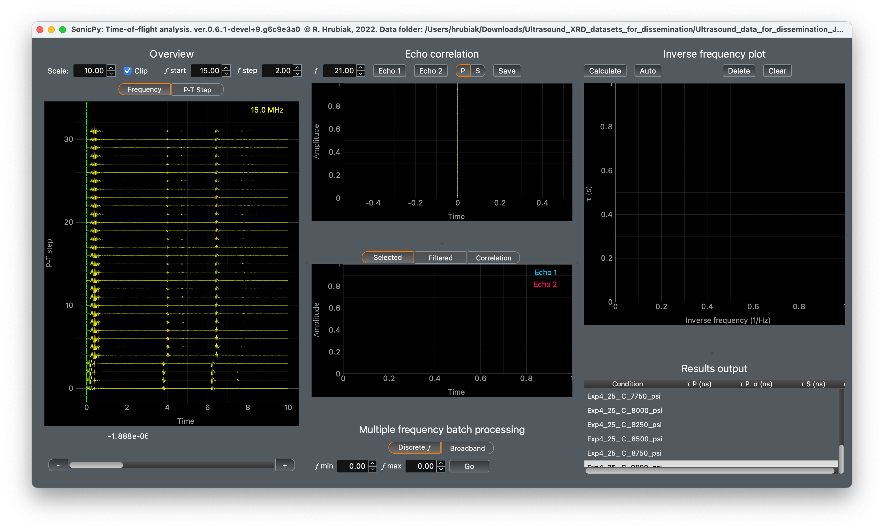
   Frequency tab shows stacked waveforms at fixed frequency and varying P-T conditions. Conversely, P-T step tab shows fixed P-T condition but varying frequencies.

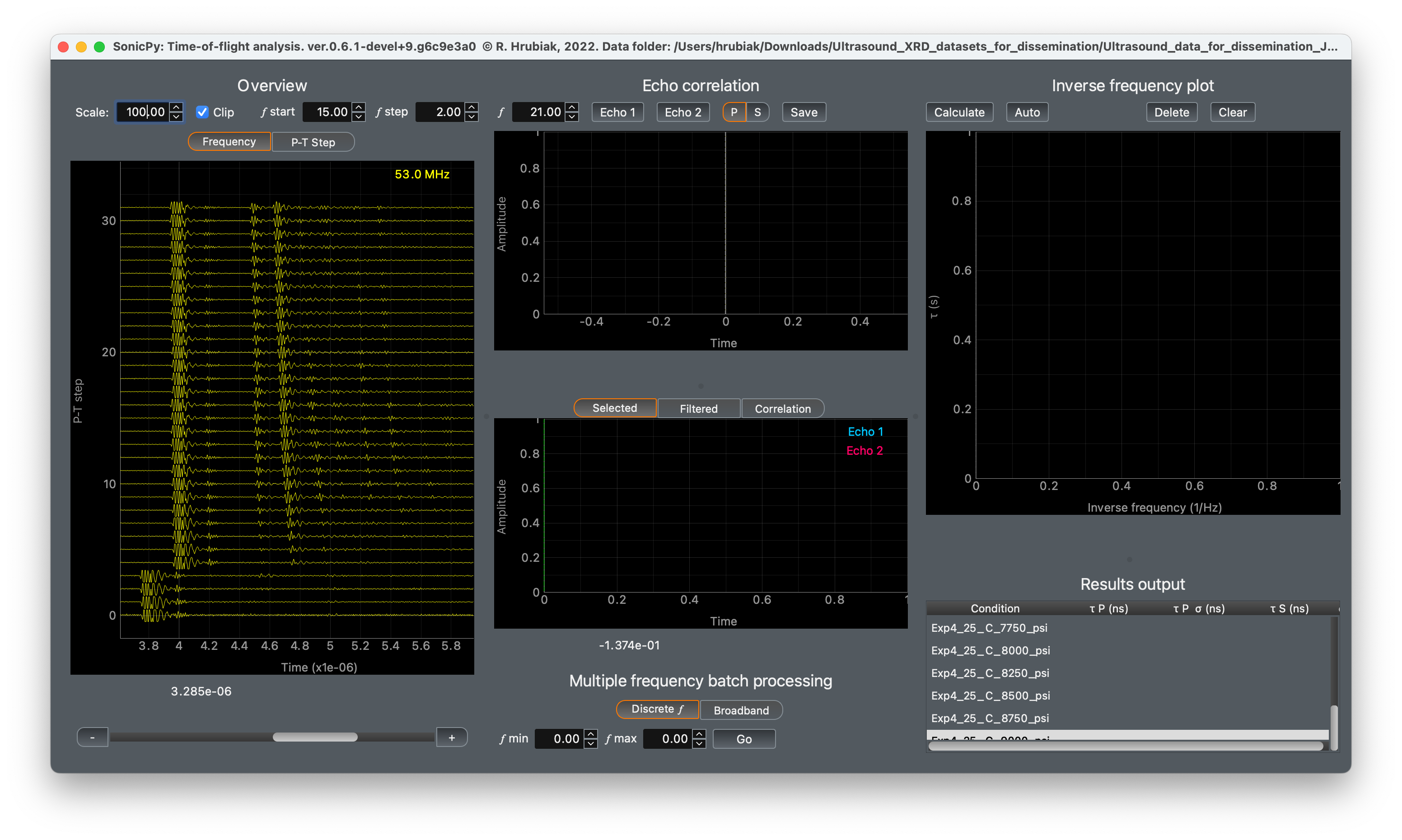
4. Adjust the Scale and use the GUI mouse interaction to zoom-in on the echoes of interest and identify the R1 and R2 echoes.

   Hint

   Hold Control key (Command key on Mac) while scrolling to adjust the Scale. Uncheck the Clip checkbox to show the full range of the singal.

   

   Note

   The scroll bar and the - + buttons underneath the Overview section can be used to change the displayed frequency or the P-T step, depending on the selected tab.

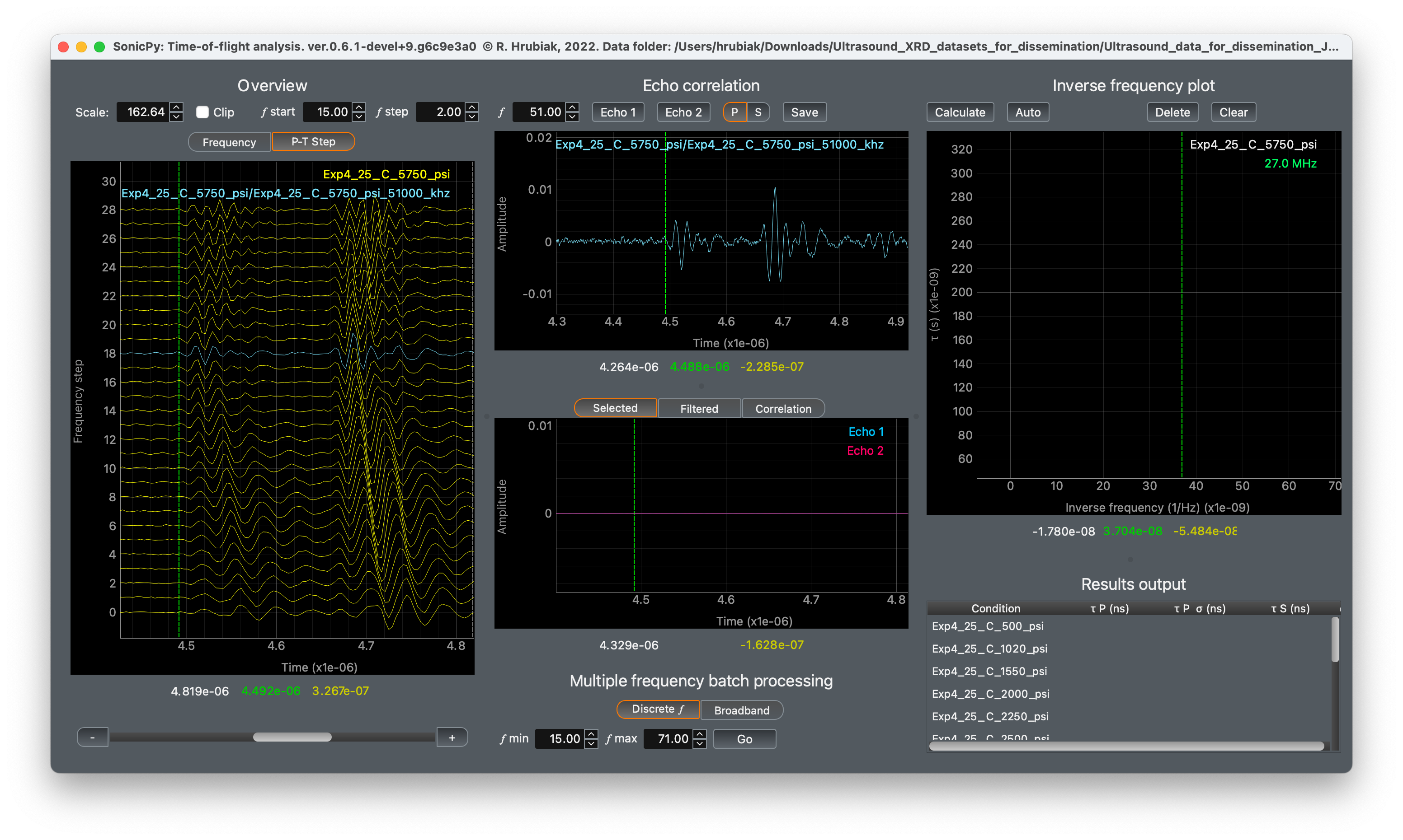
5. Click on a waveform where you have identified the R1 and R2 in order to select it. The selected waveform is displayed in the top plot of the Echo correlation section.

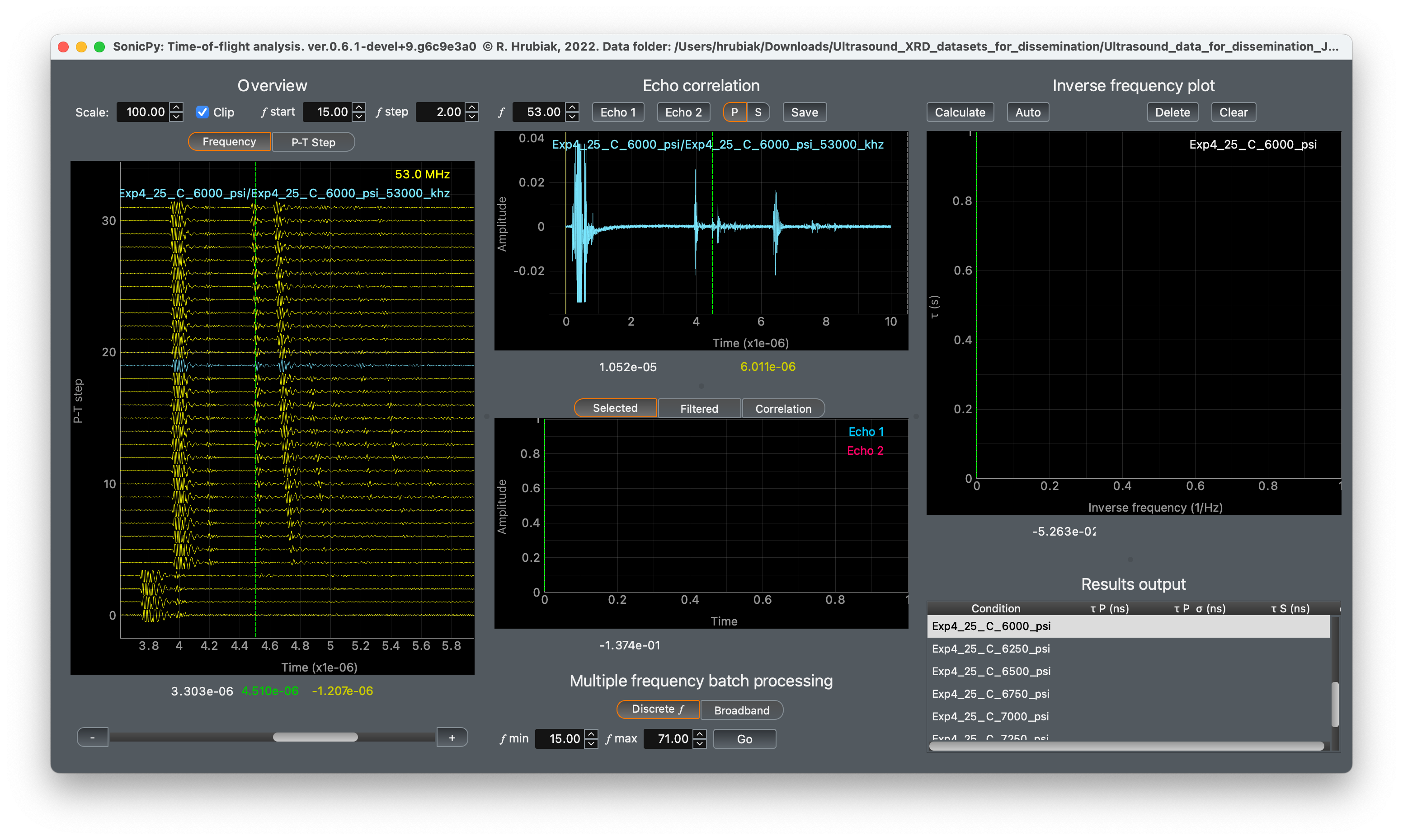
6. Use mouse left-click to position the cursor on the waveform. Select P or S at the top of the Echo correlation section for longitudinal and shear echoes, respectively. Position the cursor at the beginning of the R1 echo. Then click Echo 1.

   Note

   The cursors in the Overview and Echo correlation sections are linked, moving one will move the other.

   Hint

   Use the Frequency tab to understand which echoes are the R1 and R2 reflections. Look for echoes that have a clear pressure-dependence. At higher pressure the R1 and R2 echoes should shift to the left. At high temperatures you may see some shift as well. Conversely, other echoes, or electrical artifacts may not present a noticable pressure or temperature dependence.

   Hint

   Compressional signal is usually maximized at higher frequencies. Shear signal is usually stronger at lower frequencies.

   Hint

   The start positions of the echoes may be easier to identify by looking at the all frequencies in the P-T step tab. When you switch between Frequency and P-T step tabs, the program keeps the same waveform selected.

   

   Repeat the selection process with the R2 echo. Regions of interest will be displayed over the selected echoes in the top plot of the Echo correlation section.

   

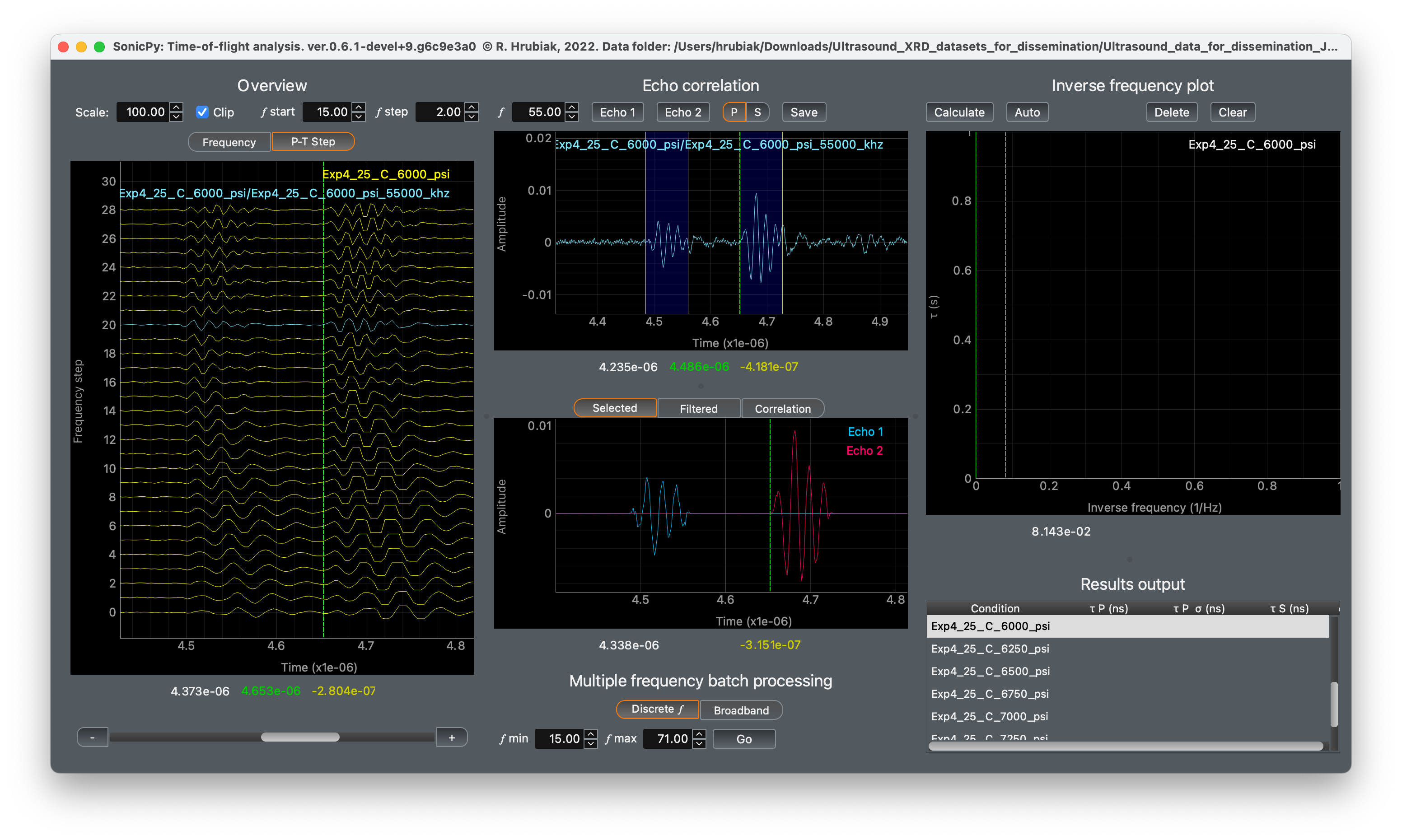
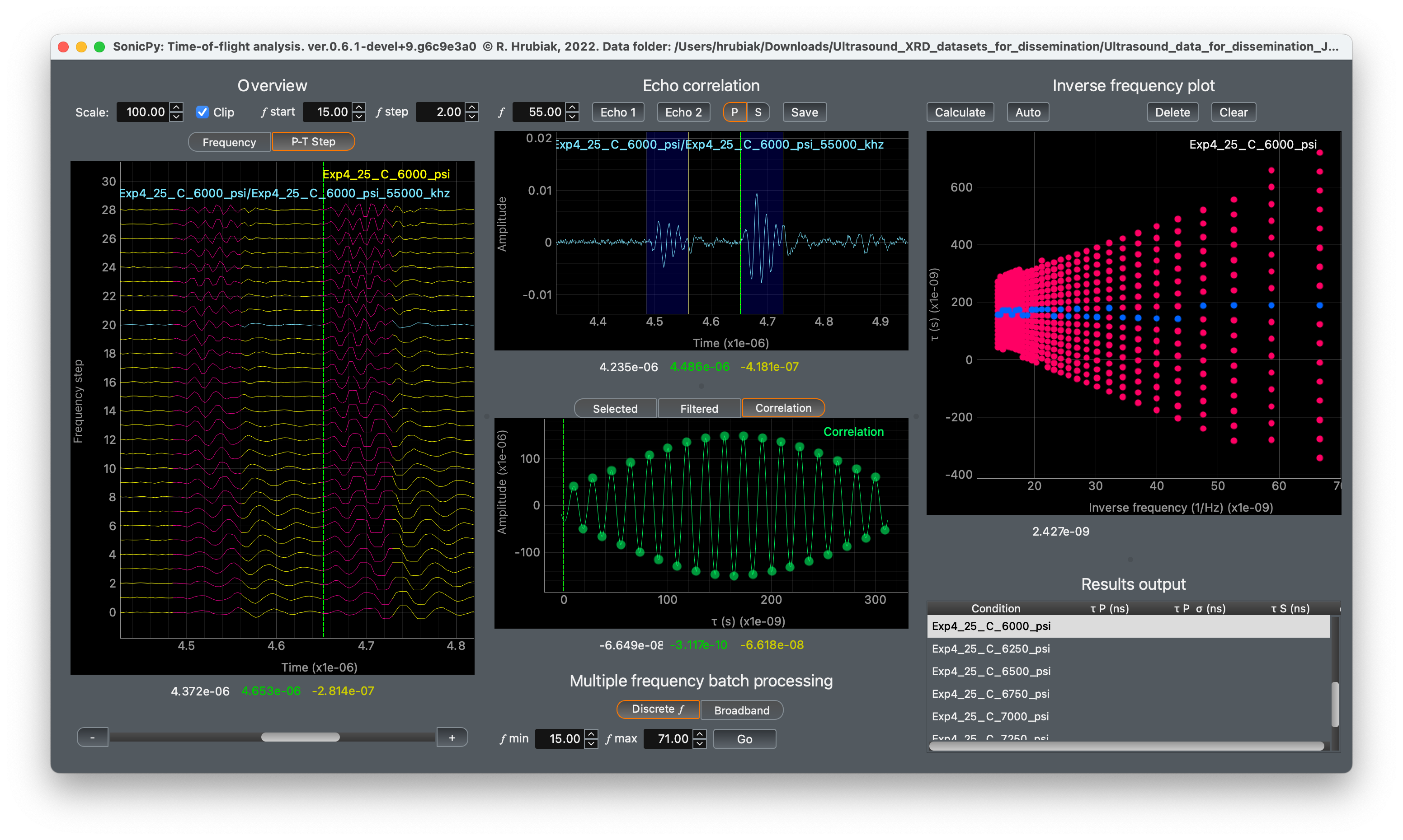
   Selected, Filetered, and Correlation tabs on the bottom of the Echo correlation section display the selected echoes, frequency filtered echoes, and the resulting correlation between the two echoes.

   Clicking Save accepts and saves the correlation result for the selected waveform.

7. Next step is to repeat this process for all the frequencies for a given P-T step.

   Manual option: select waveforms individually in the P-T step tab in the Overview section an repeat step 6 above.

   Automatic option: Click Go in the Multiple frequency batch processing section. This will process every frequency for the selected P-T step.

   The resulting correlation maxima are displayed in the Inverse frequency plot

   

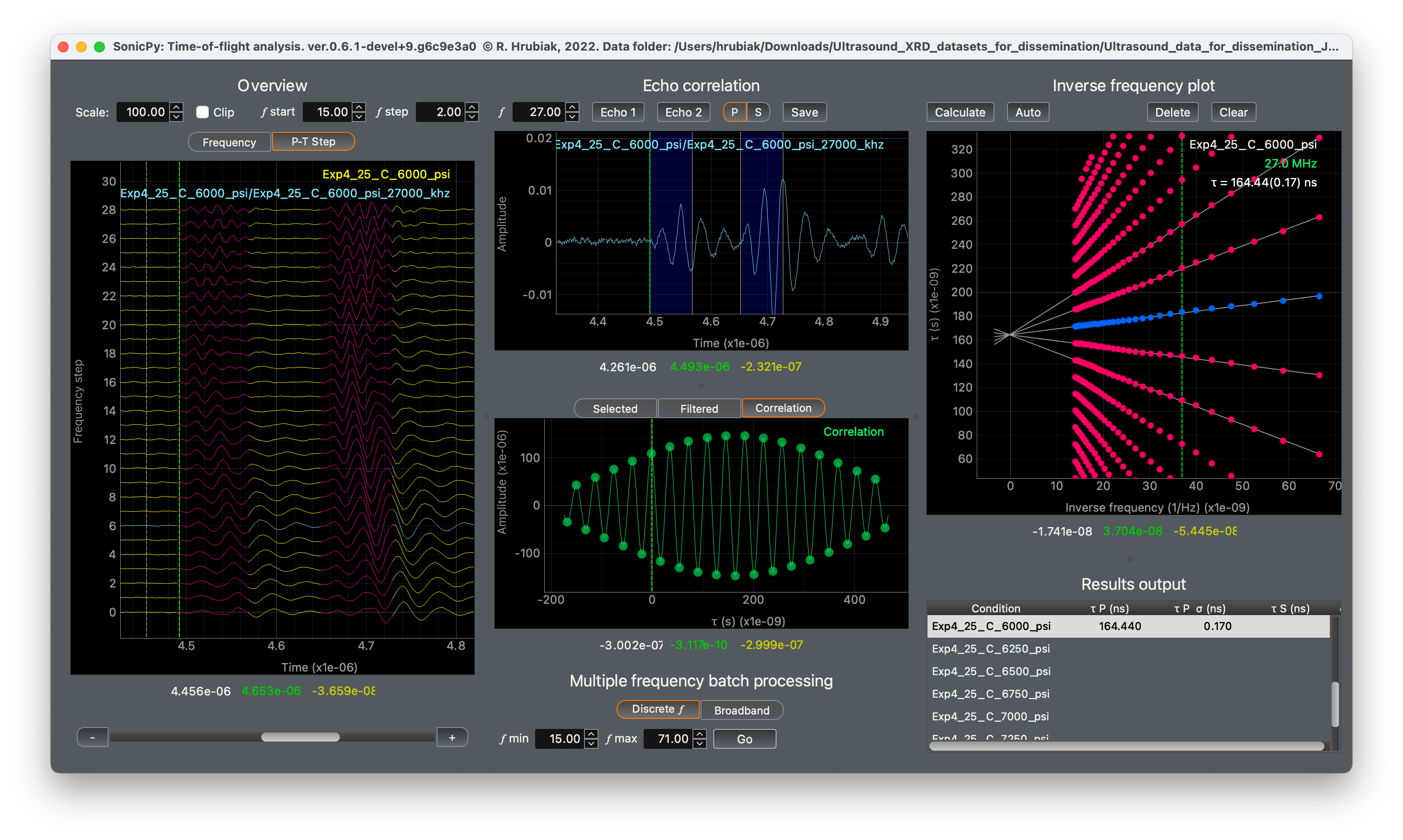
8. Click Auto in the Inverse frequency plot section. The program will select the optimal maxima, preform linear fitting, and extrapolate to the zero point in the inverse frequency domain. The y-intercept in the Inverse frequency plot corresponds to the corrected double-travel time of the sound wave. The resulting time is displayed in the top right of the Inverse frequency plot and in the Results output table section.

   

9. Zoom in on the fitted lines in the Inverse frequency plot to make sure that the fit is good. Decelect any outliers by clicking on the corresponding blue circles in the plot. Adjusting the echo positions of R1 and R2 may improve the correlation in some instances, giving a better linear fit in the Inverse frequency plot.

   

   Hint

   Changing the cursor position in the Inverse frequency plot will display the coresponding frequency in the Overview section.

10. Repeat the steps 5-9, as needed, for all the P-T steps.

11. Repeat steps 5-10, as needed, for the shear wave echoes.

    Important

    Remember to select S at the top of the Echo correlation section when working with the shear echoes.

12. Export the results table using menu File ‣ Export ‣ t results.

    The calculated time delay between R1 and R2 is the double of the travel time.

    You can calculate the sample thickness using the SonicPy: Travel-distance program. You can then use the travel-distance travel-time results to calculate the Vp and Vs.

    Note

    Data displayed in the various plots can be exported as well, in the menu File ‣ Export ‣ …